States

Lattice states in Schwinger.jl are represented by the abstract type SchwingerState, with four concrete types:

BasisState: a state specified by the eigenvalues of occupation operators $\chi^\dagger_{n,\alpha}\chi_{n,\alpha}$ and $L_0$
EDState: a linear combination of BasisStates
ITensorState: a matrix product state using ITensorMPS.jl
MPSKitState: a matrix product state using MPSKit.jl

Given a state, we can find the expectation values of the occupation operators and electric field operators:

using Schwinger
lat = Lattice(6; F = 1, a = 10) # towards the lattice strong coupling limit ga -> infty
gs = groundstate(Hamiltonian(lat; backend=:ED))

occupations(gs), electricfields(gs)

([0.9996009569748595; 0.0007976086592019167; … ; 0.9992023913407977; 0.0003990430251401046;;], [-0.0003990430251404886; 0.00039856563406142807; … ; -0.00039904302514120744; -1.1028504498522551e-15;;])

We can also evaluate the entanglement entropies of each bisection of the lattice:

using Schwinger
lat = Lattice(20; F = 1, )
gs = groundstate(Hamiltonian(lat; backend=:ITensors))
entanglements(gs)

19-element Vector{Float64}:
 0.5892661594332953
 0.394449951023898
 0.5168663014805467
 0.4537304990970688
 0.48991614664319877
 0.47010488677121676
 0.4812980874019287
 0.47489337761176054
 0.4788497809441333
 0.47593806308552933
 0.47884978094400765
 0.47489337761170825
 0.4812980874018656
 0.47010488677114726
 0.4899161466431404
 0.45373049909698143
 0.5168663014802919
 0.3944499510236873
 0.5892661594332935

When using an infinite lattice with MPSKit, we can compute these quantities in the thermodynamic limit.

using Schwinger
lat = Lattice(Inf; F = 1, )
gs = groundstate(Hamiltonian(lat; backend=:MPSKit))
entanglements(gs)

2-element Vector{Float64}:
 0.47727450642629576
 0.477274506423388

The two numbers here correspond to the two possible bisections of the two-site unit cell (corresponding to an odd and an site from the middle of a large finite lattice).

On an infinite lattice we can also probe the single-particle spectrum using the quasiparticle ansatz. For instance, at $m = 0$ the energy of the lightest quasiparticle will converge to the Schwinger boson mass $1/\sqrt{\pi} \approx 0.564$ as we take $a\to 0$:

using Schwinger
lat = Lattice(Inf; F = 1, a = 0.5, m = 0)
H = Hamiltonian(lat; backend = :MPSKit)
gs, qp = loweststates(H, 2)
real(energy(qp))   # quasiparticle mass, close to 1/√π

0.5620552417438834

The quasiparticle ansatz is a momentum eigenstate. Passing a momentum (in units of the coupling $g$, like the rest of the code) to loweststates builds the excitation at nonzero momentum — a moving quasiparticle (only available on an infinite lattice). We can then use wavepacket to build a finite-width, spatially localized packet. Here we build a packet from a quasiparticle of momentum $p = 1.0\,g$, center it on the middle 16 sites of a 64-site window, and plot its energy density relative to the vacuum (dropping the two window-boundary sites, which carry edge artifacts):

using Plots, LaTeXStrings
qp_moving = loweststates(H, 2; momentum = 1.0)[2]
wp = wavepacket(qp_moving, 64; support = 25:40)
ed = real.(energy_densities(wp))
ed = ed .- ed[5]   # subtract the (uniform) far-field vacuum value
x = (1:64) .* lat.a   # physical position of each site
plot(x[2:63], ed[2:63]; xlabel = L"x", ylabel = "Energy density above vacuum",
     legend = false, title = "Quasiparticle wavepacket (m = 0, ag = 0.5, p = 1.0g)")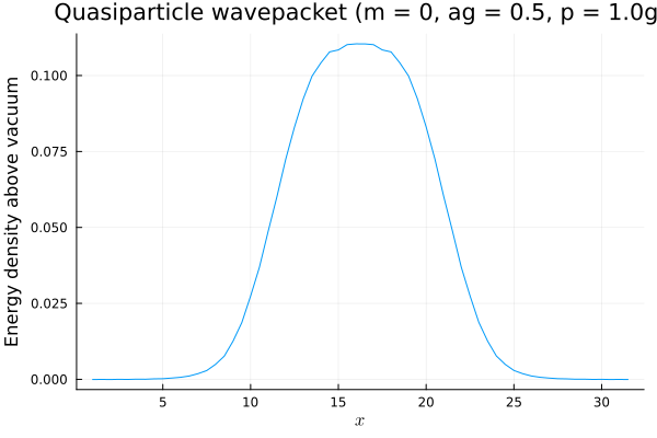

Flavor multiplets

For $F \geq 2$ flavors of equal mass, the model has a global $SU(F)$ flavor symmetry, and its excitations organize into $SU(F)$ multiplets. Passing flavor_sym = true to Lattice gauges this symmetry into the MPS (on the MPSKit backend), which lets us label an excitation by its flavor irrep and target a chosen channel with the flavor_irrep keyword of loweststates. For two flavors, the mesons split into an $SU(2)$ singlet and a triplet (flavor_singlet and flavor_adjoint), and at $m/g = 1$ the triplet is the lighter one.

We can see the triplet without any knowledge of the symmetry: exact diagonalization represents the two flavors explicitly, yet the lowest excitation comes out three-fold degenerate — an isotriplet — sitting just below a non-degenerate isosinglet.

using Schwinger
N, m, a = 8, 1.0, 1.0

# ED knows nothing about SU(2); the flavors are separate sites
Eed = sort!([real(energy(s)) for s in
             loweststates(Hamiltonian(Lattice(N; F = 2, m = m, a = a); backend = :ED), 6)])
round.(Eed .- Eed[1]; digits = 6)   # gaps above the ground state

6-element Vector{Float64}:
 0.0
 2.179603
 2.179603
 2.179603
 2.220792
 2.220792

The first three gaps are equal: the lightest excitation is a triplet. Turning on flavor_sym lets us confirm this labelling directly. We target the adjoint (the $SU(2)$ triplet, an irrep of dimension three) and singlet channels separately with flavor_irrep; the triplet is lighter, and its energy matches the ED value.

latf = Lattice(N; F = 2, m = m, a = a, flavor_sym = true)
Hf = Hamiltonian(latf; backend = :MPSKit)

E_triplet = real(energy(loweststates(Hf, 2; flavor_irrep = flavor_adjoint(latf),
                                     energy_tol = 1e-10, bonddim = 24)[2]))
E_singlet = real(energy(loweststates(Hf, 2; flavor_irrep = flavor_singlet(latf),
                                     energy_tol = 1e-10, bonddim = 24)[2]))

(E_triplet = round(E_triplet - Eed[1]; digits = 6),
 E_singlet = round(E_singlet - Eed[1]; digits = 6),
 triplet_matches_ED = isapprox(E_triplet, Eed[2]; atol = 1e-5),
 triplet_lighter = E_triplet < E_singlet)

(E_triplet = 2.179603, E_singlet = 2.24419, triplet_matches_ED = true, triplet_lighter = true)

Several other useful functions are detailed below.

Schwinger.SchwingerState — Type

SchwingerState

Abstract type for Schwinger model states.